Introduction

Sometimes, when working with scientific data, you have noisy data that you need to extract low-frequency components from.

Imagine, for example, that for a project you have recorded some audio clips that have a high-frequency "hiss" artifact from your recording equipment. Using a convolution, you can eliminate the hiss while not destroying the underlying signal that you're interested in.

png

For my current research project on an adaptive optics instrument, we needed to smooth a signal as part of our troubleshooting process to ensure we had the pattern we expected at low frequencies.

For this, we used IPython (with NumPy, SciPy, Matplotlib and friends), and AstroPy (an up-and-coming library providing implementations of common functionality for astronomers).

Open up IPython

The IPython notebook makes a lot of things easier, from keeping track of what you've tried to writing blog posts like this one. Open it up, and let's get started.

Use the magic command %pylab inline to bring the usual suspects (np, plt, etc.) into the namespace and tell IPython you want inline plots.

%pylab inline

Import the convolution functionality from AstroPy.

from astropy.convolution import convolve, Box1DKernel
# n.b. this overrides pylab's convolve()

Create a noisy signal to smooth

N = 1000 # number of samples we're dealing with
dt = 1.0 / 100.0 # 100 samples / sec

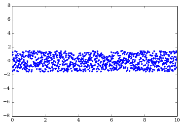
Create some nice random noise. By default, random noise is in the range [0.0, 1.0], so shift it down by 0.5 such that it's equal parts positive and negative.

noise_ts = 3 * (np.random.rand(N) - 0.5) # center at 0
plot(timesteps, noise_ts, 'b.')
ylim(-8, 8)

png

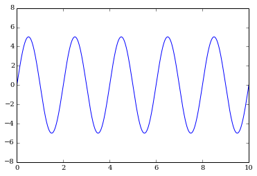
Now, we create our sine wave that we're going to mess up with noise.

A = 5.0
frequency = 0.5 # Hz
omega = 2 * np.pi * frequency
timesteps = np.linspace(0.0, N*dt, N)
signal = A * np.sin(omega * timesteps)

plot(timesteps, signal)
ylim(-8, 8)

png

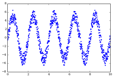
Add the noise to the signal and get a much noisier wave.

noisy_signal = noise_ts + signal

plot(timesteps, noisy_signal, 'b.')
ylim(-8, 8)

png

Smooth the noisy signal with `convolve`

Boxcar smoothing is equivalent to taking your signal %%x[t]%% and using it to make a new signal %%x'[t]%% where each element is the average of w adjacent elements. In other words, for w = 5, element %%x'[7]%% will be given by

$$ x'[7] = \frac{x[5] + x[6] + x[7] + x[8] + x[9]}{5}. $$

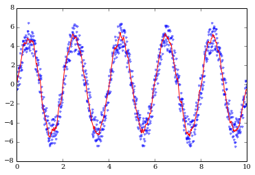
It's not perfect, but it's frequently good enough. Here we're using AstroPy's convolve function with a "boxcar" kernel of width w = 11 to eliminate the high frequency noise.

smoothed_signal = convolve(noisy_signal, Box1DKernel(11))

plot(timesteps, noisy_signal, 'b.', alpha=0.5, label="Noisy")
plot(timesteps, smoothed_signal, 'r', label="Smoothed")
ylim(-8, 8)

png

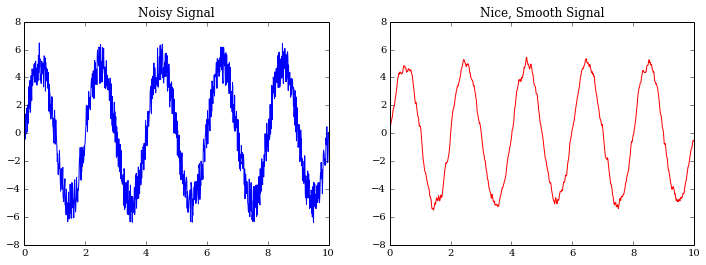
Let's make the figure we had at the beginning of this post, too.

figure(figsize=(12,4))
ax = subplot(121)
title("Noisy Signal")
plot(timesteps, noisy_signal)
xlim(0, 4)
subplot(122, sharey=ax)
title("Nice, Smooth Signal")
plot(timesteps, smoothed_signal, 'r', label="Smoothed")
xlim(0, 4)

png

Now what?

Different shaped kernels can provide useful behavior. Convolution can also be performed in two dimensions. For example, if you want to smooth an image, you can use the Box2DKernel or any of the other kernels available in AstroPy. (If you are familiar with Photoshop, the Gaussian2DKernel is analogous to the useful "Gaussian Blur" filter.)

The documentation for this part of AstroPy is particularly good, and I highly recommend reading it!

Introduction

Open up IPython

Create a noisy signal to smooth

Smooth the noisy signal with convolve

Now what?

Smooth the noisy signal with `convolve`